Gomory fractional cuts, the power of a good cut

Image by Abby Savage retrieved from Unsplash

The cutting plane method is a structured approach within mathematical optimization designed to solve Integer Linear Programming and Mixed-Integer Linear Optimization problems. It operates by first solving the continuous relaxation of the original problem and iteratively incorporating new linear constraints (termed cuts) that shrink the continuous search space without removing any feasible integer solution.

Fundamentals and historical background

Ralph E. Gomory introduced the theoretical foundations of this technique through two fundamental developments:

1. Fractional cutting plane method for pure Integer Linear Programming (Gomory, 1958).
2. Cutting plane method for Mixed-Integer Linear Programming (Gomory, 1960).

The following sections present the first method, which applies to optimization problems where all variables must be integers. This algorithm guarantees convergence to the optimal solution in a finite number of iterations. To ensure the integrality of slack variables and the mathematical validity of the process, it is essential that both, the coefficient matrix $\mathbf{A}$ and the right-hand side vector $\mathbf{b}$, contain only integer values.

Each added cut must strictly satisfy two conditions:

1. Cut off the current non-integer optimal solution from the new feasible region.
2. Be satisfied by all feasible integer solutions of the problem.

To formally construct the cut, any real number $a$ is decomposed into two components:

• Integer part $[a]$: The largest integer less than or equal to $a$.
• Fractional part $f_a$: The difference $a - [a]$, which always satisfies $0 \leqslant f_a < 1$.

For example:

• For $a = 4.67$: integer part $4$, fractional part $0.67$.
• For $a = -3.58$: integer part $-4$, fractional part $0.42$.

Derivation of the Gomory fractional cut

Let $\bar{\mathbf{x}}$ be the optimal solution obtained by solving the continuous relaxation. The set

\[\mathcal{I}_f(\bar{\mathbf{x}}) = \{s \in \mathcal{I} : f_s > 0\}\]

is defined as the set of indices associated with basic variables whose values are non-integer. If $\bar{\mathbf{x}}$ is an integer vector, then $\mathcal{I}_f(\bar{\mathbf{x}}) = \varnothing$ and the original problem is solved.

For any non-integer basic variable $x_s$ in the final Simplex tableau, the equation of the corresponding row takes the form:

\[x_s + \sum_{j \in \mathcal{J}} y_{sj} x_j = \bar{x}_s\]

Decomposing the coefficients \(y_{sj}\) and the right-hand side term \(\bar{x}_s\) into their integer and fractional parts (\(y_{sj} = [y_{sj}] + f_{sj}\) and \(\bar{x}_s = [\bar{x}_s] + f_s\)), we obtain:

\[x_s + \sum_{j \in \mathcal{J}} \big([y_{sj}] + f_{sj}\big) x_j = [\bar{x}_s] + f_s\]

Separating integer components on the left and fractional components on the right yields:

\[x_s + \sum_{j \in \mathcal{J}} [y_{sj}] x_j - [\bar{x}_s] = f_s - \sum_{j \in \mathcal{J}} f_{sj} x_j\]

Since all variables in any feasible integer solution must take integer values, the left-hand side of the equation is necessarily an integer. Consequently, the right-hand side must also be an integer. Knowing that $0 < f_s < 1$ and $f_{sj} \geqslant 0$, the following relation is derived:

\[f_s - \sum_{j \in \mathcal{J}} f_{sj} x_j \leqslant f_s < 1 \implies f_s - \sum_{j \in \mathcal{J}} f_{sj} x_j \leqslant 0\]

Rearranging the inequality defines the Gomory Fractional Cut constraint:

\[\sum_{j \in \mathcal{J}} f_{sj} x_j \geqslant f_s \iff \sum_{j \in \mathcal{J}} -f_{sj} x_j \leqslant -f_s\]

In standard form, adding the non-negative integer slack variable $w_s$, we get:

\[\sum_{j \in \mathcal{J}} -f_{sj} x_j + w_s = -f_s\]

Structure of the Gomory fractional algorithm

The algorithmic procedure follows a defined sequence:

1. Solve the continuous relaxation $P$ of the original integer problem. Let $\bar{\mathbf{x}}$ be the resulting solution.
2. While there is any non-integer basic variable ($\mathcal{I}_f(\bar{\mathbf{x}}) \neq \varnothing$):
   • Select a generating cut variable $x_s$ with $s \in \mathcal{I}_f(\bar{\mathbf{x}})$.
   • Add the cut constraint to $P$: $\sum_{j \in \mathcal{J}} f_{sj}x_j \geqslant f_s$.
   • Solve the augmented problem $P$ using the Dual Simplex Algorithm.
   • If the resulting problem is infeasible, conclude that the original integer problem is also infeasible.
   • If feasible, update $\bar{\mathbf{x}}$ with the new solution of $P$.
3. Upon reaching $\mathcal{I}_f(\bar{\mathbf{x}}) = \varnothing$, the solution $\mathbf{x} = \bar{\mathbf{x}}$ is declared as the optimal integer solution.

Criteria for selecting the cut variable

When multiple non-integer basic variables exist, the choice of cut does not affect final convergence, but it does influence the algorithm’s speed. Selecting a stronger cut eliminates a larger portion of the continuous solution space. Two main selection rules are commonly used:

• Rule 1: Select $x_s$ to minimize the ratio between the sum of the fractional parts in the row and the fractional part of the right-hand side term: \(\frac{\sum_{j \in \mathcal{J}} f_{sj}}{f_s} = \min_{i \in \mathcal{I}_f(\bar{\mathbf{x}})} \left\{ \frac{\sum_{j \in \mathcal{J}} f_{ij}}{f_i} \right\}\)

• Rule 2: Select $x_s$ whose right-hand side fractional part is maximized: \(f_s = \max_{i \in \mathcal{I}_f(\bar{\mathbf{x}})} \{ f_i \}\)

Example

Consider the following integer optimization problem:

\[\begin{align*} \min \quad & z = 4x_1 - 6x_2 \\ \text{s.t.:} \quad & -x_1 + x_2 \leqslant 1 \\ & x_1 + 3x_2 \leqslant 9 \\ & 3x_1 + x_2 \leqslant 15 \\ & x_1, x_2 \geqslant 0 \\ & x_1, x_2 \in \mathbb{Z} \end{align*}\]

Its graphical representation along with its integer feasible solutions is:

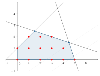
Solving the problem using the Simplex Algorithm yields the following final tableau:

\[\begin{array}{rc|rrrrr|r} & & \textcolor{gray}{4} & \textcolor{gray}{-6} & \textcolor{gray}{0} & \textcolor{gray}{0} & \textcolor{gray}{0} & \\ & & x_1 & x_2 & x_3^s & x_4^s & x_5^s & \\ \hline & z_j - c_j & 0 & 0 & -9/2 & -1/2 & 0 & -9 \\ \hline \textcolor{gray}{-6} & x_2 & 0 & 1 & 1/4 & 1/4 & 0 & 5/2 \\ \textcolor{gray}{4} & x_1 & 1 & 0 & -3/4 & 1/4 & 0 & 3/2 \\ \textcolor{gray}{0} & x_5^s & 0 & 0 & 2 & -1 & 1 & 8 \\ \hline \end{array}\]

yielding as the optimal solution (of the continuous relaxation) the point:

\[\mathbf{x}^* = (3/2,5/2,0,0,8)^\intercal \quad z^* = -9\]

Since the solution is non-integer, variable $x_2$ is selected to generate the cut. With its fractional part $f_2 = 1/2$, the fractional constraint associated with the non-basic variables $x_3^s$ and $x_4^s$ becomes: \(\frac{1}{4}x_3^s + \frac{1}{4}x_4^s \geqslant \frac{1}{2} \iff -\frac{1}{4}x_3^s - \frac{1}{4}x_4^s + x_6^s = -\frac{1}{2}\).

Adding this cut to the problem results in the following Simplex tableau:

\[\definecolor{maincolor2}{RGB}{21,182,184} \begin{array}{rc|rrrrrr|r} & & \textcolor{gray}{4} & \textcolor{gray}{-6} & \textcolor{gray}{0} & \textcolor{gray}{0} & \textcolor{gray}{0} & \textcolor{gray}{0} & \\ & & x_1 & x_2 & x_3^s & x_4^s & x_5^s & x_6^s & \\ \hline & z_j - c_j & 0 & 0 & -9/2 & -1/2 & 0 & 0 & -9 \\ \hline \textcolor{gray}{-6} & x_2 & 0 & 1 & 1/4 & 1/4 & 0 & 0 & 5/2 \\ \textcolor{gray}{4} & x_1 & 1 & 0 & -3/4 & 1/4 & 0 & 0 & 3/2 \\ \textcolor{gray}{0} & x_5^s & 0 & 0 & 2 & -1 & 1 & 0 & 8 \\ \textcolor{gray}{0} & x_6^s & 0 & 0 & -1/4 & \textcolor{maincolor2}{-1/4} & 0 & 1 & -1/2 \\ \hline \end{array}\]

and iterating using the Dual Simplex Algorithm yields the tableau:

\[\begin{array}{rc|rrrrrr|r} & & \textcolor{gray}{4} & \textcolor{gray}{-6} & \textcolor{gray}{0} & \textcolor{gray}{0} & \textcolor{gray}{0} & \textcolor{gray}{0} & \\ & & x_1 & x_2 & x_3^s & x_4^s & x_5^s & x_6^s & \\ \hline & z_j - c_j & 0 & 0 & -4 & 0 & 0 & -2 & -8 \\ \hline \textcolor{gray}{-6} & x_2 & 0 & 1 & 0 & 0 & 0 & 1 & 2 \\ \textcolor{gray}{4} & x_1 & 1 & 0 & -1 & 0 & 0 & 1 & 1 \\ \textcolor{gray}{0} & x_5^s & 0 & 0 & 3 & 0 & 1 & -4 & 10 \\ \textcolor{gray}{0} & x_4^s & 0 & 0 & 1 & 1 & 0 & -4 & 2 \\ \hline \end{array}\]

obtaining the optimal integer solution in a single iteration:

\[\mathbf{x}^* = (1, 2, 0, 2, 10, 0)^\intercal \quad z^* = -8\]

To interpret this cut in the original decision space ($x_1, x_2$), we substitute the equations for the slack variables $x_3^s = 1 + x_1 - x_2$ and $x_4^s = 9 - x_1 - 3x_2$ from the standard formulation:

\[\frac{1}{4}(1 + x_1 - x_2) + \frac{1}{4}(9 - x_1 - 3x_2) \geqslant \frac{1}{2} \iff x_2 \leqslant 2\]

that is, the Gomory fractional cut is equivalent to \(x_2 \leqslant 2\).

Geometrically, the cut in the original problem space (variables $x_1$ and $x_2$) is shown in the following figure:

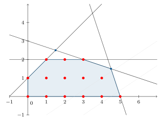
where it can be observed that the continuous solution space is reduced without removing any integer solution.

---

Ultimately, Gomory fractional cuts demonstrate the elegance of operations research: sculpting the continuous space with surgical precision to corner the integer solution without losing a single feasible point along the way.

---

Want to keep exploring the world of Operations Research? Discover more posts on the topic here.