The anatomy of a linear optimization problem

Linear optimization is much more than a tool for solving practical problems in production, logistics, or resource allocation: it is also an elegant mathematical object from a theoretical perspective.

Behind every optimal solution lie geometric and algebraic structures that allow us to understand:

• when optimal solutions exist,
• how they are reached,
• and how the entire set of feasible solutions can be described.

This post explores the fundamental concepts that support the theory of linear optimization:

• extreme points,
• extreme directions,
• how to characterize them,
• and the representation theorem for the feasible region.

The goal is to provide a clear conceptual framework that helps explain the why behind algorithms such as the Simplex method, beyond the purely mechanical computation of an optimal solution. In linear optimization, what is truly interesting is not only finding the optimum, but understanding the geometry behind it.

Notation and definitions

A linear optimization problem in standard form can be written as:

\[\begin{aligned} \min \;\; & z = \mathbf{c}^\intercal \mathbf{x} \\ \text{s.t.:}\;\; & \mathbf{A}\mathbf{x} = \mathbf{b} \\ & \mathbf{x} \geqslant \mathbf{0}. \end{aligned}\]

The feasible set is defined as:

\[\mathcal{S}=\{\mathbf{x} \in \mathbb{R}^n : \mathbf{A}\mathbf{x} = \mathbf{b},\; \mathbf{x}\geqslant \mathbf{0}\}.\]

The technical coefficient matrix \(\mathbf{A}\in\mathbb{R}^{m\times n}\) can be interpreted as a collection of $n$ vectors in \(\mathbb{R}^m\):

\[\mathbf{A} = (\mathbf{a}_1,\ldots,\mathbf{a}_n),\]

where each column is:

\[\mathbf{a}_j = \begin{pmatrix} a_{1j} \\ a_{2j} \\ \vdots \\ a_{mj} \end{pmatrix}, \qquad j=1,\ldots,n.\]

Bases and basic solutions

A common assumption in the theory is that the matrix \(\mathbf{A}\) has full row rank:

\[\mathrm{rank}(\mathbf{A}) = m.\]

In that case, there exists at least one square submatrix

\[\mathbf{B}\in\mathbb{R}^{m\times m}, \qquad |\mathbf{B}| \neq 0,\]

called a basis.

The $m$ column vectors forming the basis \(\mathbf{B}\) are linearly independent.

Choosing a basis allows us to decompose the matrix as:

\[\mathbf{A} = (\mathbf{B},\mathbf{N}),\]

which induces a natural partition of the solution vector:

\[\mathbf{x} = \begin{pmatrix} \mathbf{x}_{\mathbf{B}} \\ \mathbf{x}_{\mathbf{N}} \end{pmatrix},\]

where:

• \(\mathbf{x}_{\mathbf{B}}\in\mathbb{R}^m\) are the basic variables,
• \(\mathbf{x}_{\mathbf{N}}\in\mathbb{R}^{n-m}\) are the nonbasic variables.

Basic solution

A vector \(\mathbf{x}\in\mathbb{R}^n\) is called a basic solution if there exists a basis \(\mathbf{B}\subset\mathbf{A}\) such that the nonbasic variables are set to zero:

\[\mathbf{x} = \begin{pmatrix} \mathbf{B}^{-1}\mathbf{b} \\ \mathbf{0} \end{pmatrix}.\]

Basic feasible solution

A basic solution is called feasible if it also satisfies the nonnegativity condition:

\[\mathbf{B}^{-1}\mathbf{b}\geqslant 0.\]

Basic feasible solutions are especially important because they are directly related to the extreme points of the feasible region, as we will see next.

Convexity

One of the deepest aspects behind the theoretical analysis of linear optimization is convexity.

A nonempty set \(\mathcal{C} \subset \mathbb{R}^n\) is called convex if:

\[\lambda \mathbf{x} + (1-\lambda)\mathbf{y} \in \mathcal{C} \qquad \forall \mathbf{x},\mathbf{y}\in\mathcal{C},\; \forall \lambda\in[0,1].\]

Geometrically, this means that for any two points in the set, the line segment joining them remains entirely inside the set.

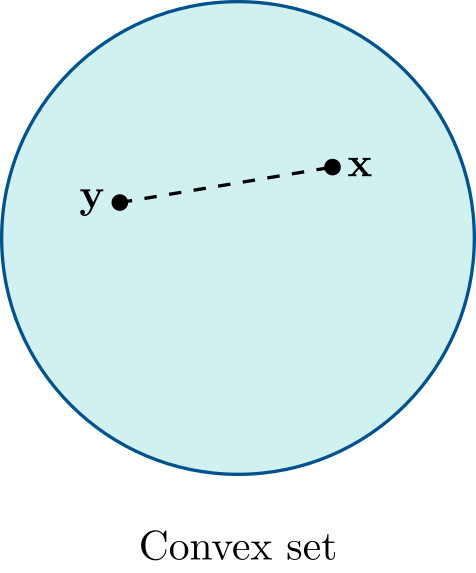
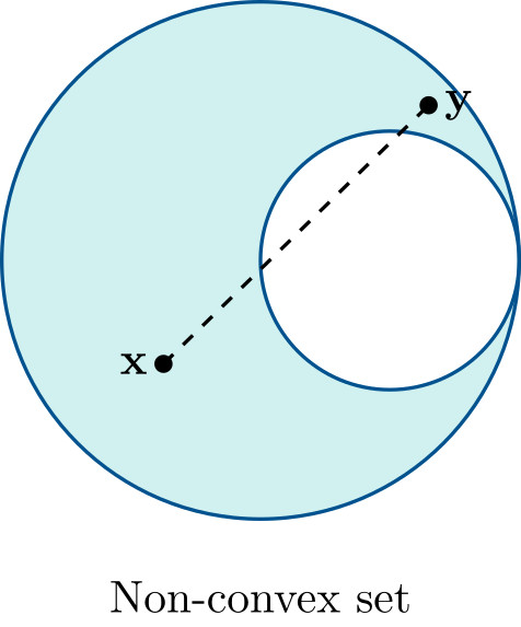
The feasible set of a linear optimization problem,

\[\mathcal{S}=\{\mathbf{x}\in\mathbb{R}^n:\mathbf{A}\mathbf{x}=\mathbf{b},\;\mathbf{x}\geqslant 0\},\]

is a convex set.

Extreme points

Although \(\mathcal{S}\) contains infinitely many points, its structure is determined by a much smaller collection of special elements: the extreme points, which correspond to the “vertices” of the feasible polytope.

If an optimal solution exists, then it can be found at an extreme point.

For this reason, it is essential to understand what extreme points are and how they can be characterized.

Given a convex set \(\mathcal{C}\subset\mathbb{R}^n\), a point \(\mathbf{x}\in\mathcal{C}\) is called an extreme point if:

\[\mathbf{x}=\lambda\mathbf{y}+(1-\lambda)\mathbf{z}, \;0<\lambda<1, \;\mathbf{y},\mathbf{z}\in\mathcal{C} \Rightarrow\] \[\mathbf{x}=\mathbf{y}=\mathbf{z}.\]

In other words, an extreme point cannot be expressed as a convex combination of two distinct points in the set.

Characterization of extreme points

Let \(\mathcal{S}=\{\mathbf{x}\in\mathbb{R}^n:\mathbf{A}\mathbf{x}=\mathbf{b},\;\mathbf{x}\geqslant 0\},\) where \(\mathbf{A}\in\mathbb{R}^{m\times n}\) and \(\mathrm{rank}(\mathbf{A})=m\). Then:

\(\bar{\mathbf{x}}\) is an extreme point of \(\mathcal{S}\) if and only if

\(\exists\,\mathbf{B}\subset\mathbf{A}\) such that \(|\mathbf{B}|\neq 0, \;\mathbf{B}^{-1}\mathbf{b}\geqslant 0.\)

In that case:

\[\bar{\mathbf{x}}= \begin{pmatrix} \mathbf{B}^{-1}\mathbf{b}\\ \mathbf{0} \end{pmatrix}.\]

The number of extreme points is bounded by:

\[\binom{n}{m}.\]

If $\mathcal{S} \neq \emptyset$, then at least one extreme point exists.

Extreme directions

In problems with unbounded feasible regions, we encounter extreme directions, which describe how the feasible set can extend infinitely.

A nonzero vector \(\mathbf{d}\neq 0\) is a direction of a convex set \(\mathcal{C}\) if:

\[\forall\mathbf{x}\in\mathcal{C},\; \forall\mu\geqslant 0 \Rightarrow \mathbf{x}+\mu\mathbf{d}\in\mathcal{C}.\]

Two directions \(\mathbf{d}^1\) and \(\mathbf{d}^2\) are equivalent if \(\mathbf{d}^1=\alpha\mathbf{d}^2,\; \alpha>0.\)

In linear optimization,

Given the feasible set $\mathcal{S}={\mathbf{x} \in \mathbb{R}^n : \mathbf{A}\mathbf{x} = \mathbf{b}, \mathbf{x} \geqslant \mathbf{0}}$, we have:

\(\mathbf{d}\) is a direction of \(\mathcal{S}\) if and only if \(\mathbf{d} \geqslant 0,\; \mathbf{d}\neq 0,\; \mathbf{A}\mathbf{d}=0.\)

Given a convex set $\mathcal{C}$, a direction $\mathbf{d}$ is called an extreme direction if whenever:

\[\mathbf{d} = \mu_1 \mathbf{d}^1 + \mu_2 \mathbf{d}^2,\]

with $\mu_1,\mu_2>0$ and $\mathbf{d}^1,\mathbf{d}^2$ directions of $\mathcal{C}$, then:

\[\mathbf{d} \simeq \mathbf{d}^1 \simeq \mathbf{d}^2.\]

Extreme directions can also be characterized.

Characterization of extreme directions

Let $\mathcal{S}={\mathbf{x} \in \mathbb{R}^n : \mathbf{A}\mathbf{x} = \mathbf{b}, \mathbf{x} \geqslant \mathbf{0}}$, where $\mathbf{A}$ is an $m\times n$ matrix with $\mathrm{rank}(\mathbf{A})=m$. Then:

$\mathbf{d}$ is an extreme direction of $\mathcal{S}$ if and only if there exists a basis $\mathbf{B}\subset\mathbf{A}$ with $|\mathbf{B}|\neq 0$ such that $\mathbf{A}=(\mathbf{B},\mathbf{N}),$ and there exists a column $\mathbf{a}_j\in\mathbf{N}$ satisfying $\mathbf{B}^{-1}\mathbf{a}_j\leqslant 0,$ so that $\mathbf{d}=\alpha\mathbf{d}^0$ with $\alpha>0$ and:

\[\mathbf{d}^0=\begin{pmatrix}-\mathbf{B}^{-1} \mathbf{a}_j \\ \mathbf{e}_j\end{pmatrix},\]

where $\mathbf{e}_j$ is the vector with all components zero except the $j$-th, which equals 1.

The number of extreme directions is bounded by:

\[\binom{n}{m+1}.\]

Representation Theorem

The representation theorem is a consequence of several classical results in convex geometry thanks to the works of Minkowski, Carathéodory, Steinitz, Weyl and Motzkin ((Minkowski, 1897), (Carathéodory, 1907), (Steinitz, 1916), (Weyl, 1935), (Motzkin, 1936)), established even before the birth of linear optimization as a discipline.

Representation Theorem

Let $\mathcal{S}={\mathbf{x} \in \mathbb{R}^n : \mathbf{A}\mathbf{x} = \mathbf{b}, \mathbf{x} \geqslant \mathbf{0}}$, where $\mathbf{A}$ is an $m\times n$ matrix with $\mathrm{rank}(\mathbf{A})=m$.
Let ${\mathbf{x}^1,\ldots,\mathbf{x}^k}$ be the set of extreme points of $\mathcal{S}$ and ${\mathbf{d}^1,\ldots,\mathbf{d}^l}$ its extreme directions. Then:

\[\mathbf{x} \in \mathcal{S} \Leftrightarrow \wedge \begin{cases} \exists (\lambda_1,\ldots,\lambda_k) & \lambda_i \geqslant 0,\; \sum_{i=1}^k \lambda_i = 1 \\ \exists (\mu_1,\ldots,\mu_l) & \mu_j \geqslant 0 \end{cases}\]

such that:

\[\mathbf{x} = \sum_{i=1}^k \lambda_i \mathbf{x}^i + \sum_{j=1}^l \mu_j \mathbf{d}^j.\]

This theorem shows that every feasible solution can be expressed entirely in terms of extreme points and extreme directions. To do so, one must identify these sets using the characterization results presented above.

Examples

Consider the feasible region (independent of the objective function) of a linear optimization problem, written in standard form by adding slack variables:

\[\begin{aligned} -x_1 + x_2 & \leqslant 2 \\ x_1 - 2x_2 & \leqslant 2 \\ x_1, x_2 & \geqslant 0 \end{aligned} \qquad \begin{aligned} -x_1 + x_2 + x_3^h & = 2 \\ x_1 - 2x_2 + x_4^h & = 2 \\ x_1, x_2, x_3^h, x_4^h & \geqslant 0 \end{aligned}\]

This problem has three extreme points:

\[\mathbf{x}_1 = \begin{pmatrix}0 \\ 0 \\ 2 \\ 2\end{pmatrix} \qquad \mathbf{x}_2 = \begin{pmatrix}2 \\ 0 \\ 4 \\ 0\end{pmatrix} \qquad \mathbf{x}_3 = \begin{pmatrix}0 \\ 2 \\ 0 \\ 6\end{pmatrix}\]

and two extreme directions:

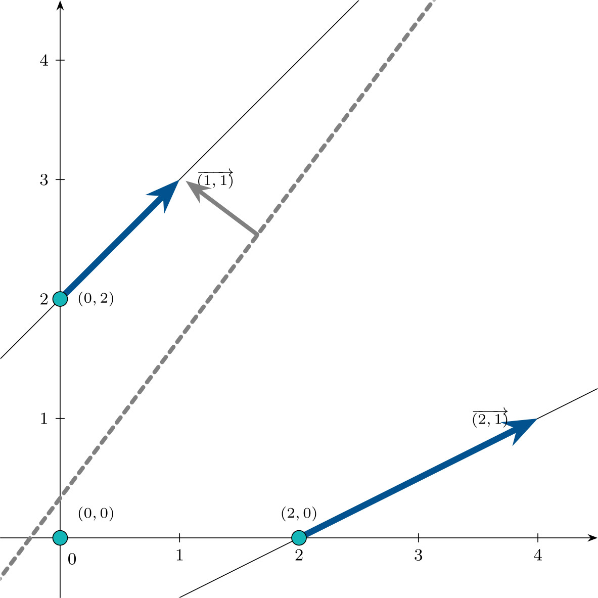
\[\mathbf{d}_1 = \begin{pmatrix}1 \\ 1 \\ 0 \\ 1\end{pmatrix} \qquad \mathbf{d}_2 = \begin{pmatrix}2 \\ 1 \\ 1 \\ 0\end{pmatrix}\]

represented in the following figure in $\mathbb{R}^2$:

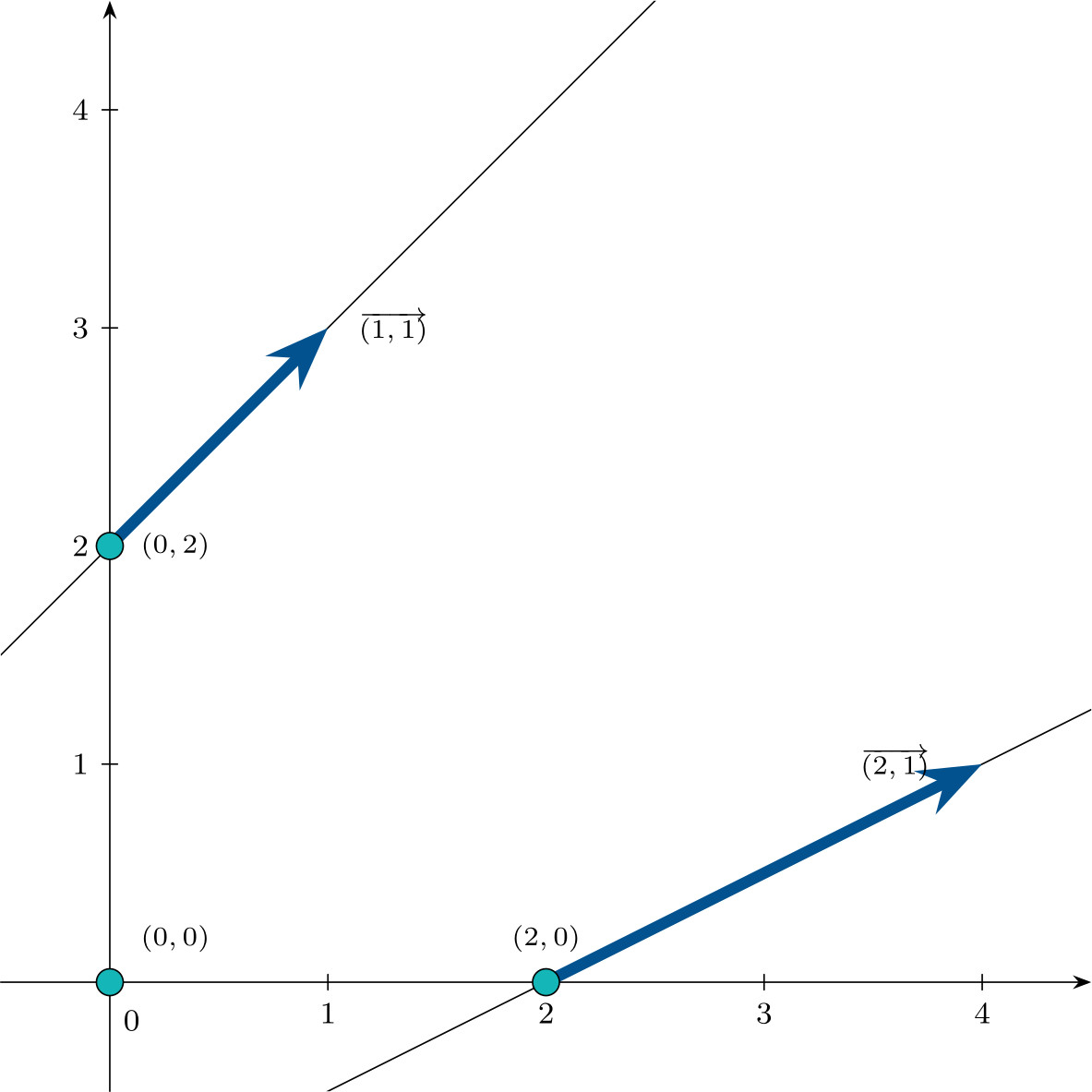
Using the representation theorem, the set $\mathcal{S}$ can be written as:

\[\begin{aligned} \mathcal{S} =\Biggl\{ &\lambda_1 \begin{pmatrix} 0\\0\\2\\2 \end{pmatrix} +\lambda_2 \begin{pmatrix} 2\\0\\4\\0 \end{pmatrix} +\lambda_3 \begin{pmatrix} 0\\2\\0\\6 \end{pmatrix} +\mu_1 \begin{pmatrix} 1\\1\\0\\1 \end{pmatrix} +\mu_2 \begin{pmatrix} 2\\1\\1\\0 \end{pmatrix} :\; \\[0.4em] & \lambda_1+\lambda_2+\lambda_3=1, \lambda_1,\lambda_2,\lambda_3\geqslant 0, \qquad \mu_1,\mu_2\geqslant 0 \Biggr\}. \end{aligned}\]

Consequences of the representation theorem

The representation theorem allows us to classify the different types of solutions of a minimization linear optimization problem.

• The problem is unbounded if there exists an extreme direction $\mathbf{d}^j$ such that $\mathbf{c}^\intercal \mathbf{d}^j < 0$.

• The problem has an optimal solution if all extreme directions satisfy $\mathbf{c}^\intercal \mathbf{d}^j \geqslant 0$, or if no extreme directions exist, and the optimum is attained at an extreme point.

Resolution procedure and combinatorics

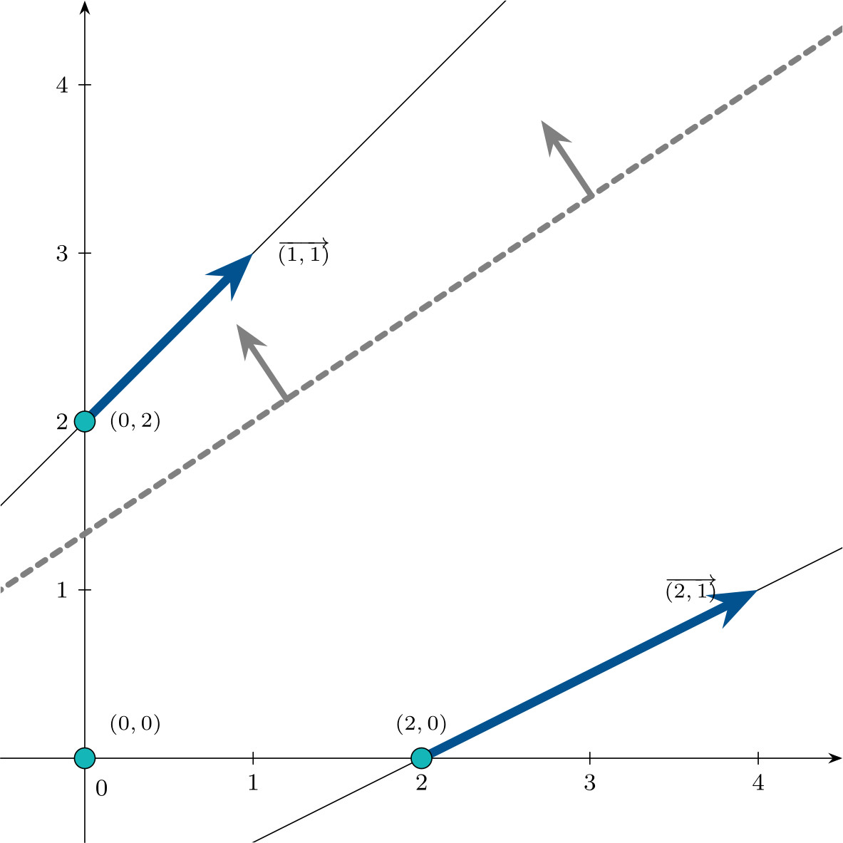
Using the same feasible region, we now analyze different cost vectors, which lead to different objective functions and therefore different types of solutions.

• $\mathbf{c}^\intercal = (2,-3,0,0)$

\[\mathbf{c}^\intercal \mathbf{d}^1 = (2,-3,0,0)\begin{pmatrix}1 \\ 1 \\ 0 \\ 1\end{pmatrix} = -1 < 0,\]

so the problem is unbounded.

• $\mathbf{c}^\intercal = (4,-3,0,0)$

Since \(\mathbf{c}^\intercal \mathbf{d}^1 \geqslant 0\) and \(\mathbf{c}^\intercal \mathbf{d}^2 \geqslant 0,\)

the problem has an optimal solution, attained at the vertex with minimum objective value, namely $\mathbf{x}^3$ (where \(\mathbf{c}^\intercal \mathbf{x}^3 = -6\)).

• $\mathbf{c}^\intercal = (0,1,0,0)$

Again, \(\mathbf{c}^\intercal \mathbf{d}^1 \geqslant 0\) and \(\mathbf{c}^\intercal \mathbf{d}^2 \geqslant 0,\)

so the problem has an optimal solution. In this case, two vertices attain the same minimum value: $\mathbf{x}^1$ and $\mathbf{x}^2$, with

\[\mathbf{c}^\intercal \mathbf{x}^1 = \mathbf{c}^\intercal \mathbf{x}^2 = 0.\]

The set of optimal solutions is:

\[\left\{\lambda\begin{pmatrix}0 \\ 0 \\ 2 \\ 2\end{pmatrix} + (1-\lambda)\begin{pmatrix}2 \\ 0 \\ 4 \\ 0\end{pmatrix}, \;\; \lambda \in [0,1]\right\}.\]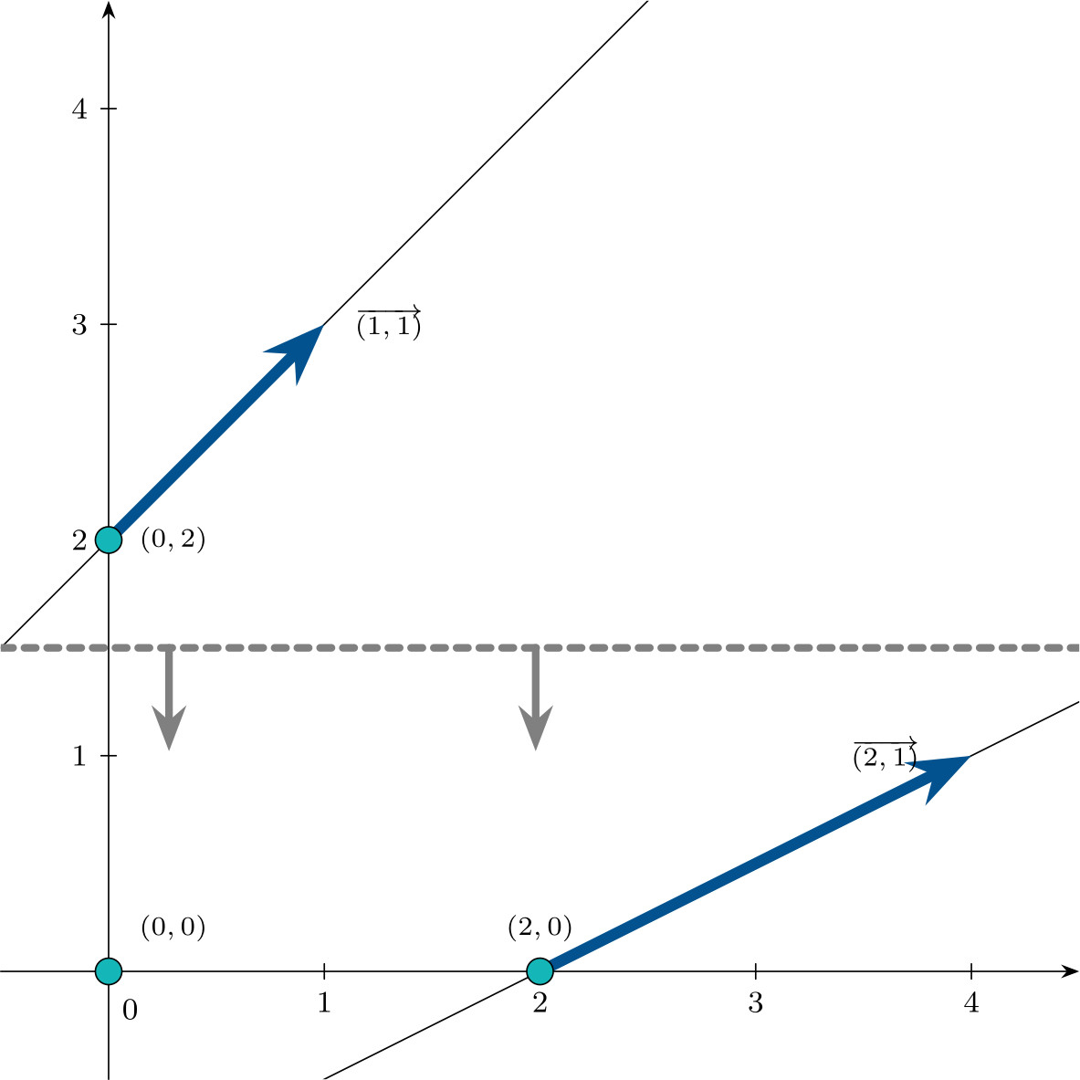

• $\mathbf{c}^\intercal = (1,-1,0,0)$

Since \(\mathbf{c}^\intercal \mathbf{d}^1 \geqslant 0\) and \(\mathbf{c}^\intercal \mathbf{d}^2 \geqslant 0,\)

the problem has an optimal solution. Evaluating the vertices, the minimum is attained at $\mathbf{x}^3$, where \(\mathbf{c}^\intercal \mathbf{x}^3 = -2.\)

The set of optimal solutions is:

\[\left\{\begin{pmatrix}0 \\ 2 \\ 0 \\ 6\end{pmatrix} + \mu\begin{pmatrix}1 \\ 1 \\ 0 \\ 1\end{pmatrix}, \;\; \mu \geqslant 0 \right\}.\]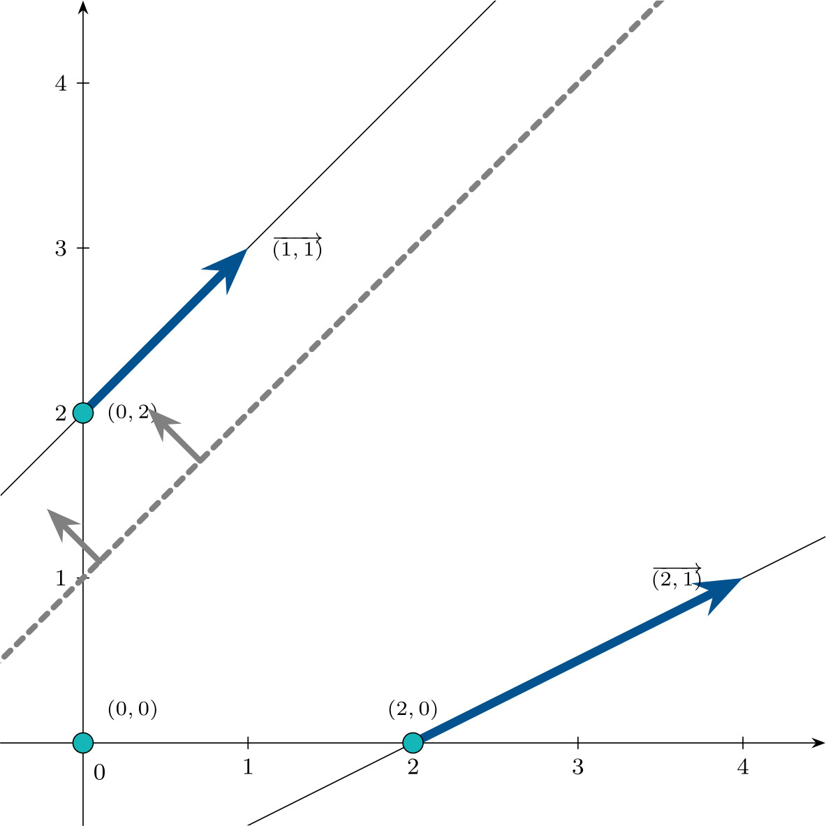

Combinatorics

The combinatorial growth of all possible bases becomes extremely fast. Even for moderate dimensions, such as $n=40$ and $m=20$, we obtain:

\[\binom{40}{20}=137,846,528,820.\]

Although enumerating all extreme points and extreme directions is not practical for large-scale problems due to this combinatorial explosion, the theoretical analysis provides the essential foundations: it reveals the geometric structure of the feasible region, characterizes the possible types of solutions, and ultimately motivates the development of efficient algorithms such as the Simplex method, which exploits precisely these properties.

References

- NPKAllgemeine Lehrsätze üuber die convexen PolyederNachrichten von der Gesellschaft der Wissenschaften zu Göttingen, Mathematisch-Physikalische Klasse, Dec 1897
- Math. Ann.Über den Variabilitätsbereich der Koeffizienten von Potenzreihen, die gegebene Werte nicht annehmenMathematische Annalen, Dec 1907
- Chap. BookEncyclopädie der mathematischen Wissenschaften, vol. III.1.2 (Geometrie), Chap. IIIAB12Dec 1916
- CMH
- PhD Thesis
Enjoy Reading This Article?
Here are some more articles you might like to read next: